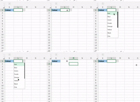
Dynamic Drop-down List - Stop scrolling to search for options in the list.

Excel Data validation provides a wonderful feature of limiting the response to standard/specific options. However this feature becomes bothersome when the list becomes too large to scroll through.

Well if you have faced this issue too, this blog is just perfect for you!

LETS MAKE THAT LIST REDUCE THE OPTIONS BASED ON WHAT YOU ARE TYPING!

Yes it is possible to do that!

Well to do this we need to break down the whole procedure into multiple steps.

Step 1: Unique List

We will generate a list of unique fields for our drop down.

To do that we can use Unique Functions (as shown in the B column below). To make sure that any criteria added in the list in the future is also captured, we will select the whole column (A:A). However, this can give us an additional field 0, due to empty cells in the selected A column.

To tackle this we will use the Filter function (as shown in the C column below). Here we are stating that give us the

A	B	C
Red	=Unique(A:A)	​=FILTER(UNIQUE(A:A),UNIQUE(A:A)<>"")
Blue
Black
Brown

Now that we have a unique list of options, we can proceed to Step 2.

Step 2: Searching for our input

Now that we have our unique list, the next step is to make this list searchable.

We have our unique list in the C column, so hereon we will refer to the C column whenever we are referring to our unique list.

Now we will search for the input in the E column inside our list. To do that we will use the Find function, as shown below.

If you are wondering what is # in the formula. We use # to tell the formula to spill it over to all the cells used by our Unique formula.

Now Find formula will give us some error whenever it cannot find a match, so lets change it true and false output. How? we will use ISNUMBER (as shown in D2).

C	D	E
Red	​=FIND(E1,C1#,1)	e
Blue	​=ISNUMBER(FIND(E1,C1#,1))
Black
Brown

The output in the D column will look like as shown in D Column below. What it is telling us which color contains "e". If it is True in D1, means color in C1 cell contains "e". In this case C1 = Red, hence it is true and so on.

​C	D	E
Red	TRUE	e
​Blue	TRUE
Black	FALSE
Brown	FALSE

Step 3: Obtaining only the True Match

We will use the Filter function (as shown below) once again to get only the True matches. Check below table.

=FILTER(C1#,ISNUMBER(FIND(E1,C1#,1))=TRUE(),C1#)

D	E	F
Red	e
Blue

Now we have a list which contains the sub string mentioned in the E column.

Now that if you understand the above steps., let's put everything inside a single formula which will look like this;

=FILTER(FILTER(UNIQUE(A:A),UNIQUE(A:A)<>""),ISNUMBER(FIND(L1,FILTER(UNIQUE(A:A),UNIQUE(A:A)<>""),1))=TRUE(),FILTER(UNIQUE(A:A),UNIQUE(A:A)<>""))

Seems intimidating, but that is how good it is. For much easier understanding here is the code

=FILTER(

FILTER(UNIQUE(A:A),UNIQUE(A:A)>""),

ISNUMBER(FIND(E1,FILTER(UNIQUE(A:A),UNIQUE(A:A)<>""),1))=TRUE(),

FILTER(UNIQUE(A:A),UNIQUE(A:A)<>"")

)

Lets say we have our unique list in C column, then formula reduces to

=FILTER(C1#,ISNUMBER(FIND(E1,C1#,1))=TRUE(),C1#)

Step 4: Data Validation list

Note that this is a formula based list, hence list updates only after cell value is updated, thus to do that, we need to make sure that the "Show Alert" under "Error Alert" is unchecked.

Note - Pic is downloaded from the internet.

Now you can enter a value in the data validation, then click outside and when you are back at it, you will see a filtered list.

Now the question is that it defeats the purpose of data validation since a user is able to update the field with any value, then what can we do?

What we can do is we can use a cell as a search field (say F Column) which will filter the list in data validation in the E column (with show error selected). Check below.

D	E	F
Red	Drop down	Enter text to search
Blue		e

Check below to see how it works.

Thanks for reading. If you have any doubt or query, do write back and we will try to SOLVE THAT QUERY.